GIFT tutorial for advanced users
Pierre Denelle & Patrick Weigelt
2024-12-02
Source:vignettes/GIFT_advanced_users.Rmd
GIFT_advanced_users.Rmd![]()

This vignette documents some functions and specificities that were not presented in the main vignette of the package. It is mainly intended for advanced users of the GIFT database.
1. Versions and metadata for checklists
All functions in the package have a version argument.
This argument allows you to retrieve different instances of the GIFT
database and thus make all previous studies using the GIFT database
reproducible. For example, the version used in Weigelt et al. (2020) is
"1.0". To get more information about the contents of the
different versions, you can go here and click on the
Version Log tab.
To access all the available versions of the database, you can run the following function:
versions <- GIFT_versions()
kable(versions, "html") %>%
kable_styling(full_width = FALSE)| ID | version | description | taxonomy | phylogeny | overlap |
|---|---|---|---|---|---|
| 1 | 1.0 | 2018-08-08: Data included in and workflows used to assemble GIFT 1.0 are described in detail in: Weigelt, P., König, C. & Kreft, H. (2020) GIFT – A Global Inventory of Floras and Traits for macroecology and biogeography. Journal of Biogeography, 47, 16-43. doi: 10.1111/jbi.13623 | The Plant List 1.1 and resources used by TNRS at the time | NA | gaptani (version: okt2005, ID_column: UNITID); glonaf (version: 2017-06-12; ID_column: OBJIDsic); gmba (version: 1.0, ID_column: rownames) |
| 2 | 2.0 | 2019-09-01: New checklist and trait data included for Europe, the Mediterranean, temperate Asia, Panama, Japan, Java, New Zealand, Easter Island and the Torres Strait Islands. Updated workflows to document biases in the distribution of trait data; Updated taxonomic trait derivation; Final trait values and agreement scores for trait values from several resources are now calculated separately including and excluding restricted resources. | The Plant List 1.1 and resources used by TNRS at the time | NA | gaptani (version: okt2005, ID_column: UNITID); glonaf (version: 2017-06-12; ID_column: OBJIDsic); gmba (version: 1.0, ID_column: rownames) |
| 3 | 2.1 | 2021-05-21: New checklists and traits included for the Americas, Crimea, Madagascar, Arabian peninsula, Laos, Bhutan, India, China, Sunda-Sahul shelf, Tonga, Canary Islands, West Africa and for ferns and palms globally. Large categorical trait data included from Try. | The Plant List 1.1 and resources used by TNRS at the time | NA | gaptani (version: okt2005, ID_column: UNITID); glonaf (version: 2017-06-12; ID_column: OBJIDsic); gmba (version: 1.0, ID_column: rownames) |
| 4 | 2.2 | 2022-05-30: New checklists (with a focus on endemic species) and traits for various oceanic archipelagos (Cook Islands, Madeira, Arctic Islands, Cayman Islands, Comores, Juan Fernandez, Palau, Galapagos, Frisian Islands, Antilles, Japan, Mayotte, Fiji, Taiwan, etc.) and various mainland regions (Equatorial Guinea and the entire former USSR in sub-regions). | The Plant List 1.1 and resources used by TNRS at the time | NA | gaptani (version: okt2005, ID_column: UNITID); glonaf (version: 2017-06-12; ID_column: OBJIDsic); gmba (version: 1.0, ID_column: rownames) |
| 5 | 3.0 | 2023-06-30: New data and updated workflows as described in: Denelle, P., Weigelt, P. & Kreft, H. (2023) GIFT - an R package to access the Global Inventory of Floras and Traits. BioRxiv, doi: 10.1101/2023.06.27.546704. Updated workflows include: (1) New taxonomic name standardization based on WCVP; (2) More statistics on species level trait aggregation; (3) Updated extraction of raster layer values per GIFT region and new raster resources; (4) Updated phylogeny. | World Checklist of Vascular Plants (WCVP, v9) and resources used by TNRS at the time | Phylogeny built using U.PhyloMaker R-package (Jin & Qian, 2022) based on the GBOTB megatree from Smith & Brown (2018) and Zanne et al. (2014), standardized according to WCVP. | gaptani (version: okt2005, ID_column: UNITID); glonaf (version: 2021-07-02; ID_column: OBJIDsic); gmba (version: 1.2, ID_column: rownames) |
| 6 | 3.1 | 2023-11-11: New checklist data for Mongolia and Farasan Archipelago and correction of seed traits for Hawaii (ref 16; units). | World Checklist of Vascular Plants (WCVP, v9) and resources used by TNRS at the time | Phylogeny built using U.PhyloMaker R-package (Jin & Qian, 2022) based on the GBOTB megatree from Smith & Brown (2018) and Zanne et al. (2014), standardized according to WCVP. | gaptani (version: okt2005, ID_column: UNITID); glonaf (version: 2021-07-02; ID_column: OBJIDsic); gmba (version: 2.0, ID_column: GMBA_V2_ID) |
| 7 | 3.2 | 2024-06-13: New oceanic archipelago trait data and global parasitism information | World Checklist of Vascular Plants (WCVP, v9) and resources used by TNRS at the time | Phylogeny built using U.PhyloMaker R-package (Jin & Qian, 2022) based on the GBOTB megatree from Smith & Brown (2018) and Zanne et al. (2014), standardized according to WCVP. | gaptani (version: okt2005, ID_column: UNITID); glonaf (version: 2021-07-02; ID_column: OBJIDsic); gmba (version: 2.0, ID_column: GMBA_V2_ID) |
The version column of this table is the one to use if
you want to retrieve past versions of the GIFT database. By default, the
argument used is GIFT_version = "latest" which leads to the
current latest stable version of the database (“2.0” in October
2022).
The GIFT_lists() function can be run to retrieve
metadata about the GIFT checklists. In the next chunk, we call it with
different values for the GIFT_version argument.
list_latest <- GIFT_lists(GIFT_version = "latest") # default value
list_1 <- GIFT_lists(GIFT_version = "1.0")
The number of available checklists was 3122 in the version 1.0 and equals 4475 in the version 2.0.
2. References
When using the GIFT database in a research article, it is a good
practice to cite the references used, and list them in an Appendix. The
following function retrieves the reference for each checklist, as well
as some metadata. References are documented in the ref_long
column.
ref <- GIFT_references()
ref <- ref[which(ref$ref_ID %in% c(22, 10333, 10649)),
           c("ref_ID", "ref_long", "geo_entity_ref")]

# 3 first rows of that table
kable(ref, "html") %>%
kable_styling(full_width = FALSE)| ref_ID | ref_long | geo_entity_ref | |
|---|---|---|---|
| 22 | 22 | Kirchner, Picot, Merceron & Gigot (2010) Flore vasculaire de La Réunion. Conservatoire Botanique National de Mascarin, Réunion; France. | La Réunion |
| 667 | 10333 | Zizka (1991) Flowering plants of Easter Island. Palmarum hortus francofurtensis 3, 3-108. | Easter Island |
| 880 | 10649 | Pavlov (1954-1966) Flora Kazakhstana. Nauka Kazakhskoy SSR, Alma-Ata, Kazakhstan. | Kazakhstan |
The next chunk describes the steps to retrieve the publication sources when you start from specific regions, let’s say the Canary islands.
# List of all regions
regions <- GIFT_regions()

# Example
can <- 1036 # entity ID for Canary islands

# What references
gift_lists <- GIFT_lists()

can_ref <- gift_lists[which(gift_lists$entity_ID %in% c(can)), "ref_ID"]

# What sources
kable(ref[which(ref$ref_ID %in% can_ref), ], "html") %>%
kable_styling(full_width = TRUE)| ref_ID | ref_long | geo_entity_ref |
|---|---|---|
3. Checklist data
The main wrapper function for retrieving checklists and their species
composition is GIFT_checklists() but you can also retrieve
individual checklists using GIFT_checklists_raw(). You
would need to know the identification number list_ID of the
checklists you want to retrieve.
To quickly see all the
list_ID available in the database, you can run
GIFT_lists() as shown in Section
1.
When calling GIFT_checklists_raw(), you can set the
argument namesmatched to TRUE in order to get
additional columns informing about the taxonomic harmonization that was
performed when the list was uploaded to the GIFT database.
listID_1 <- GIFT_checklists_raw(list_ID = c(11926))
listID_1_tax <- GIFT_checklists_raw(list_ID = c(11926), namesmatched = TRUE)

ncol(listID_1) # 16 columns
ncol(listID_1_tax) # 33 columns
length(unique(listID_1$work_ID)); length(unique(listID_1_tax$orig_ID))
In the list we called up, you can see that we “lost” some species
after the taxonomic harmonization since we went from 1331 in the source
to 1106 after the taxonomic harmonization. This means that several
species were considered as synonyms or unknown plant species in the
taxonomic backbone used for harmonization.
Note: the main
service used for taxonomic harmonization of species names was
The Plant List up to version 2.0 and World checklist of Vascular
Plants afterwards.
4. Spatial subset
In the main vignette, we illustrated how to retrieve checklists that fall into a provided shapefile, using the western Mediterranean basin provided with the GIFT R package.
data("western_mediterranean")Here we provide more details on the different values the
overlap argument can take, using the
GIFT_spatial() function. The following figure illustrates
how this argument works:

Figure 1. GIFT spatial
We now illustrate this by retrieving checklists falling in the western Mediterranean basin using the four options available.
med_centroid_inside  <- GIFT_spatial(shp = western_mediterranean,
                                     overlap = "centroid_inside")
med_extent_intersect <- GIFT_spatial(shp = western_mediterranean,
                                     overlap = "extent_intersect")
med_shape_intersect <- GIFT_spatial(shp = western_mediterranean,
                                    overlap = "shape_intersect")
med_shape_inside <- GIFT_spatial(shp = western_mediterranean,
                                 overlap = "shape_inside")
length(unique(med_extent_intersect$entity_ID))
length(unique(med_shape_intersect$entity_ID))
length(unique(med_centroid_inside$entity_ID))
length(unique(med_shape_inside$entity_ID))
We see here that we progressively lose lists as we apply more
selective criterion on the spatial overlap. The most restrictive option
being overlap = "shape_inside" with 72 regions, then
overlap = "centroid_inside" with 84 regions,
overlap = "shape_intersect" with 104 regions and finally
the less restrictive one being overlap = "extent_intersect"
with 108 regions.
Using the functions GIFT_shapes()
and calling it for the entity_IDs retrieved in each instance, we can
download the shape files for each region.
geodata_extent_intersect <- GIFT_shapes(med_extent_intersect$entity_ID)

geodata_shape_inside <-
  geodata_extent_intersect[which(geodata_extent_intersect$entity_ID %in%
                                   med_shape_inside$entity_ID), ]
geodata_centroid_inside <-
  geodata_extent_intersect[which(geodata_extent_intersect$entity_ID %in%
                                   med_centroid_inside$entity_ID), ]
geodata_shape_intersect <-
  geodata_extent_intersect[which(geodata_extent_intersect$entity_ID %in%
                                   med_shape_intersect$entity_ID), ]
And then make a map.
par_overlap <- par(mfrow = c(2, 2), mai = c(0, 0, 0.5, 0))
plot(sf::st_geometry(geodata_shape_inside),
     col = geodata_shape_inside$entity_ID,
     main = paste("shape inside\n",
                  length(unique(med_shape_inside$entity_ID)),
                  "polygons"))
plot(sf::st_geometry(western_mediterranean), lwd = 2, add = TRUE)

plot(sf::st_geometry(geodata_centroid_inside),
     col = geodata_centroid_inside$entity_ID,
     main = paste("centroid inside\n",
                  length(unique(med_centroid_inside$entity_ID)),
                  "polygons"))
points(geodata_centroid_inside$point_x, geodata_centroid_inside$point_y)
plot(sf::st_geometry(western_mediterranean), lwd = 2, add = TRUE)

plot(sf::st_geometry(geodata_shape_intersect),
     col = geodata_shape_intersect$entity_ID,
     main = paste("shape intersect\n",
                  length(unique(med_shape_intersect$entity_ID)),
                  "polygons"))
plot(sf::st_geometry(western_mediterranean), lwd = 2, add = TRUE)

plot(sf::st_geometry(geodata_extent_intersect),
     col = geodata_extent_intersect$entity_ID,
     main = paste("extent intersect\n",
                  length(unique(med_extent_intersect$entity_ID)),
                  "polygons"))
plot(sf::st_geometry(western_mediterranean), lwd = 2, add = TRUE)
par(par_overlap)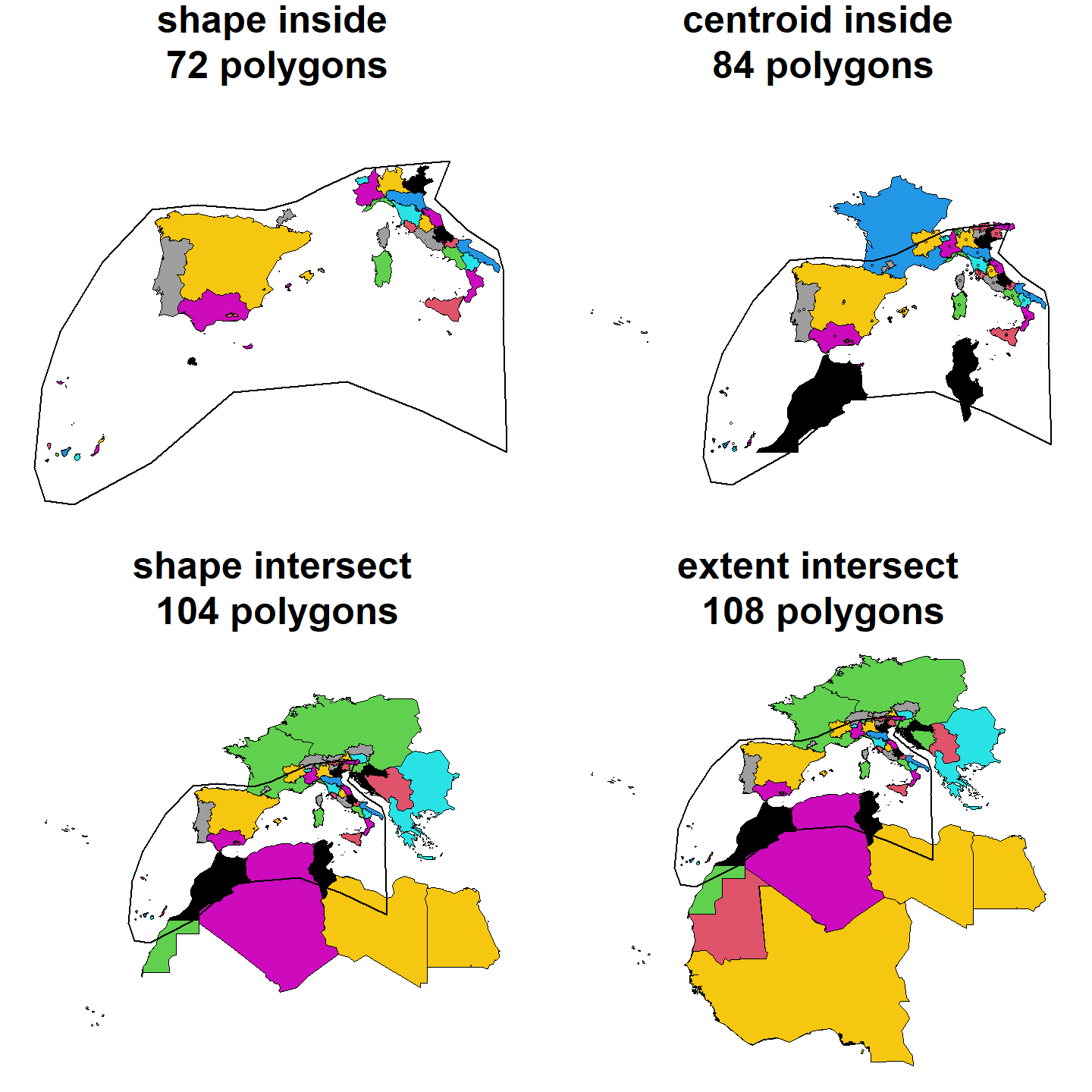
5. Remove overlapping regions
GIFT comprises many polygons and for some regions, there are several polygons overlapping. How to remove overlapping polygons and the associated parameters are two things detailed in the main vignette. We here provide further details:
length(med_shape_inside$entity_ID)## [1] 72
length(GIFT_no_overlap(med_shape_inside$entity_ID, area_threshold_island = 0,
                       area_threshold_mainland = 100, overlap_threshold = 0.1))
## [1] 53
# The following polygons are overlapping:
GIFT_no_overlap(med_shape_inside$entity_ID, area_threshold_island = 0,
                area_threshold_mainland = 100, overlap_threshold = 0.1)
## [1] 145 146 147 148 149 150 151 414 415 416 417 547
## [13] 548 549 550 551 552 586 591 592 736 738 739 10001
## [25] 10072 10104 10184 10303 10422 10430 10978 11029 11030 11031 11033 11035
## [37] 11038 11039 11042 11044 11045 11046 11434 11474 11477 11503 12231 12232
## [49] 12233 12632 12633 12634 12635
# Example of two overlapping polygons: Spain mainland and Andalusia
overlap_shape <- GIFT_shapes(entity_ID = c(10071, 12078))
par_overlap_shp <- par(mfrow = c(1, 1))
plot(sf::st_geometry(overlap_shape),
     col = c(rgb(red = 1, green = 0, blue = 0, alpha = 0.5),
             rgb(red = 0, green = 0, blue = 1, alpha = 0.3)),
     lwd = c(2, 1),
     main = "Overlapping polygons")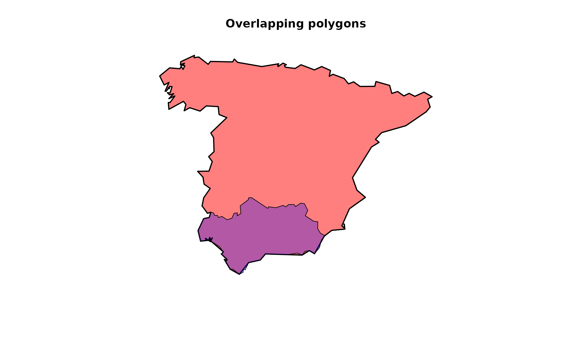
par(par_overlap_shp)

GIFT_no_overlap(c(10071, 12078), area_threshold_island = 0,
                area_threshold_mainland = 100, overlap_threshold = 0.1)
## [1] 12078
GIFT_no_overlap(c(10071, 12078), area_threshold_island = 0,
                area_threshold_mainland = 100000, overlap_threshold = 0.1)
## [1] 100715.2. By ref_ID
In GIFT_checklists(), there is also the possibility to
remove overlapping polygons only if they belong to the same reference
(i.e. same ref_ID).
We show how this works with the following example:
ex <- GIFT_checklists(taxon_name = "Tracheophyta", by_ref_ID = FALSE,
                      list_set_only = TRUE, GIFT_version = "3.0")
ex2 <- GIFT_checklists(taxon_name = "Tracheophyta",
                       remove_overlap = TRUE, by_ref_ID = TRUE,
                       list_set_only = TRUE, GIFT_version = "3.0")
ex3 <- GIFT_checklists(taxon_name = "Tracheophyta",
                       remove_overlap = TRUE, by_ref_ID = FALSE,
                       list_set_only = TRUE, GIFT_version = "3.0")

length(unique(ex$lists$ref_ID)) # 369 checklists
length(unique(ex2$lists$ref_ID)) # 364 checklists
length(unique(ex3$lists$ref_ID)) # 336 checklists
Asking for checklists of vascular plants, we get 369 checklists
without any overlapping criterion, 336 if we remove overlapping polygons
and 364 if we remove overlapping polygons at the reference level.
So what is the difference between the second and third case?
Let’s look at the checklists that are present in the second example but
not in the third.
28 references are in the second example (overlapping regions removed
at the reference level) and not in the third (all overlapping regions
removed). If we look at one of the listed references
ref_ID = 10143, we see that it is a checklist for the
Pilbara region in Australia. Its entity_ID is 10043.
Looking at the GIFT web site, we see that other regions can overlap with
it.
# Pilbara region Australy and overlapping shapes
pilbara <- GIFT_shapes(entity_ID = c(10043, 12172, 11398, 11391, 10918))
ggplot(pilbara) +
  geom_sf(aes(fill = as.factor(entity_ID)), alpha = 0.5) +
  scale_fill_brewer("entity_ID", palette = "Set1")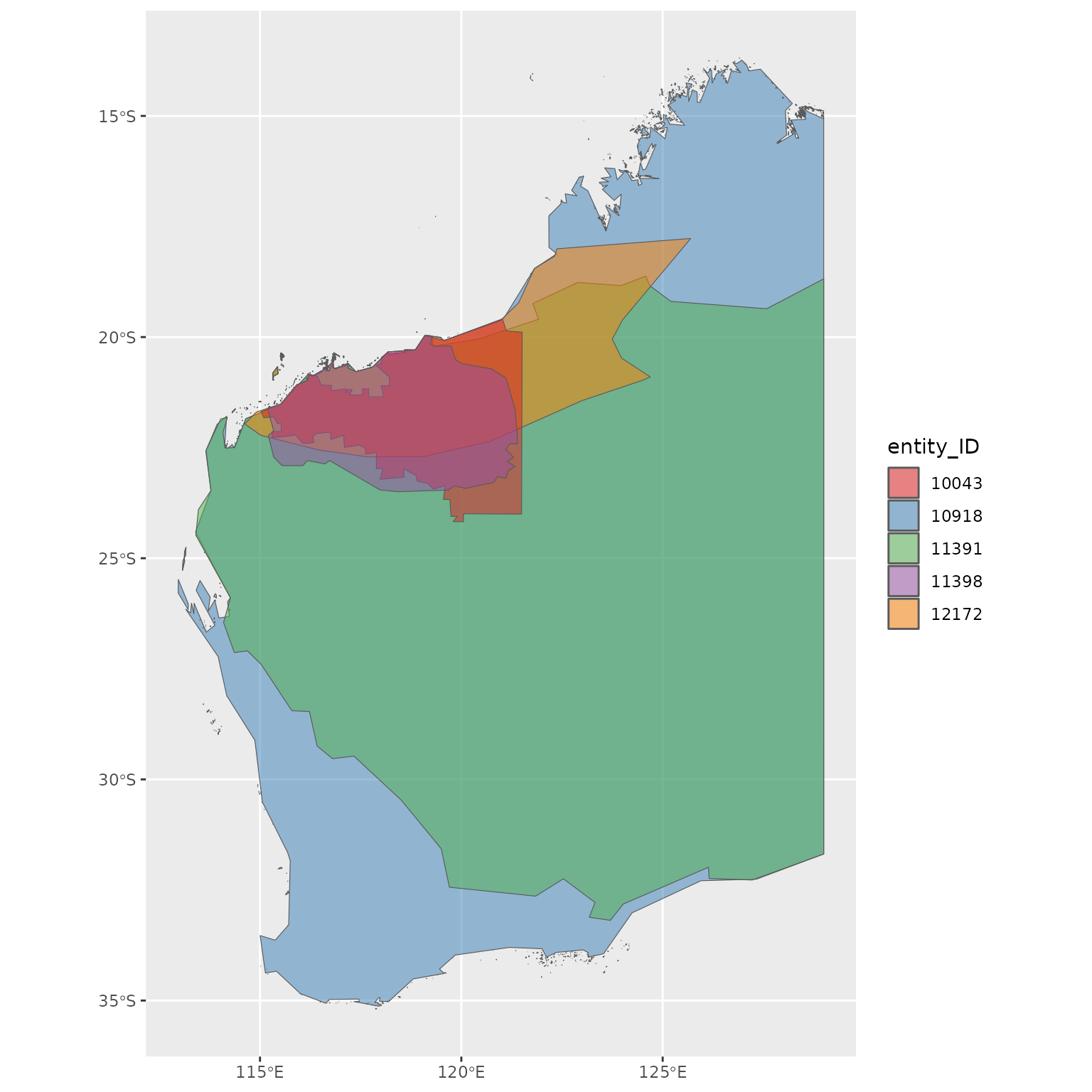
Since these polygons do not belong to the same ref_ID,
they are kept if by_ref_ID = TRUE but are removed if
by_ref_ID = FALSE.
6. Species
All the plant species present in the GIFT database can be retrieved
using GIFT_species().
species <- GIFT_species()To add additional information, like their order or family, we can
call GIFT_taxgroup().
# Add Family
species$Family <- GIFT_taxgroup(
  as.numeric(species$work_ID), taxon_lvl = "family", return_ID = FALSE,
  species = species)
Order or higher levels can also be retrieved.
GIFT_taxgroup(as.numeric(species$work_ID[1:5]), taxon_lvl = "order",
              return_ID = FALSE)
GIFT_taxgroup(as.numeric(species$work_ID[1:5]),
              taxon_lvl = "higher_lvl", return_ID = FALSE,
              species = species)
As mentioned above, plant species names may vary from the original
sources they come from to the final work_species name they
get, due to the taxonomic harmonization procedure. Looking up a species
and the different steps of taxonomic harmonization is possible with the
GIFT_species_lookup() function.
Fagus <- GIFT_species_lookup(genus = "Fagus", epithet = "sylvatica",
                             namesmatched = TRUE)
In this table, we can see that the first entry Fagus silvatica was later changed to the accepted name Fagus sylvatica.
6.2. Retrieve work_IDs for external species list
sp_list <- c("Anemone nemorosa", "Fagus sylvatica")

gift_sp <- GIFT_species()

sapply(sp_list, function(x) grep(x, gift_sp$work_species))
gift_sp[sapply(sp_list, function(x) grep(x, gift_sp$work_species)), ]

# With fuzzy matching
# library("fuzzyjoin")
# library("dplyr")
sp_list <- data.frame(work_species = c("Anemona nemorosa", "Fagus sylvaticaaa"))

fuzz <- stringdist_join(sp_list, gift_sp,
                        by = "work_species",
                        mode = "left",
                        ignore_case = FALSE,
                        method = "jw",
                        max_dist = 99,
                        distance_col = "dist")

fuzz %>%
  group_by(work_species.x) %>%
  slice_min(order_by = dist, n = 1)
7. Taxonomy
The taxonomy used in GIFT database can be downloaded using
GIFT_taxonomy().
taxo <- GIFT_taxonomy()8. Overlap_GloNAF tables (and others)
Since other global databases of plant diversity exist and may be
based on different polygons, we provide a function
GIFT_overlap() than can look at the spatial overlap between
GIFT polygons and polygons coming from other databases.
So far,
only two resources are available: glonaf and
gmba. glonaf stands for Global
Naturalized Alien Flora and gmba for Global Mountain Biodiversity
Assessment.
GIFT_overlap() returns the spatial overlap in percent
for each pairwise combination of polygons between GIFT and the other
resource.
Let’s illustrate this with the GMBA shapefile.
gmba_overlap <- GIFT_overlap(resource = "gmba")

kable(gmba_overlap[1:5, ], "html") %>%
kable_styling(full_width = FALSE)| entity_ID | gmba_ID | overlap12 | overlap21 |
|---|---|---|---|
| 12094 | 12159 | 0.1783509 | 0.7623728 |
| 12094 | 11134 | 0.0060051 | 0.9985861 |
| 12094 | 12218 | 0.1398757 | 0.7948085 |
| 12094 | 16791 | 0.0301742 | 0.9385561 |
| 12094 | 16809 | 0.0036777 | 0.9566831 |
We see that two overlap columns are returned: overlap12
and overlap21.
The first column returns the overlap between the GIFT region and the
other resource. The second column returns the overlap between the other
resource and the GIFT region.
For example, if we look at the polygon 11861 of GIFT:
gmba_overlap[which(gmba_overlap$entity_ID == 11861 &
                     gmba_overlap$gmba_ID == 731), ]
## [1] entity_ID gmba_ID overlap12 overlap21
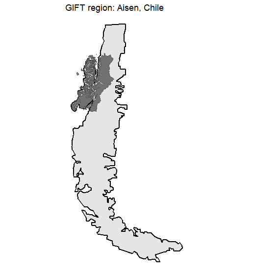
## <0 rows> (or 0-length row.names)The corresponding region is the Aisen province in Chile and it
overlaps at 95% with the GMBA polygon number 731.
At the same time the GMBA polygon 731 only overlaps at 13% with the
Aisen province of Chile.
This is because the corresponding mountain region is larger than the
GIFT region and encompasses it as we can see on this plot (the dark
polygon is the GIFT region):
9. Plotting phylogeny for a specific region
We here want to plot the phylogenetic tree of native plant species occurring in Tenerife island.
# List table
gift_list <- GIFT_lists()
# Tenerife data for the following list_IDs: 150, 14110, 14228

# Retrieve the lists
tenerife <- GIFT_checklists_raw(list_ID = c(150, 14110, 14228))

# Extract unique native species only
tenerife_sp <- tenerife[which(tenerife$native == 1), ] %>%
  dplyr::select(work_species) %>%
  distinct(.keep_all = TRUE)

# Harmonizing species names between the species table and the phylogeny
tenerife_sp$work_species <- gsub(" ", "_", tenerife_sp$work_species,
                                 fixed = TRUE)

# Phylogeny
phy <- GIFT_phylogeny()

# Dropping tips
tenerife_phy <- ape::keep.tip(
  phy,
  tip = phy$tip.label[(phy$tip.label %in% tenerife_sp$work_species)])

plot(tenerife_phy, type = "fan", cex = 0.2)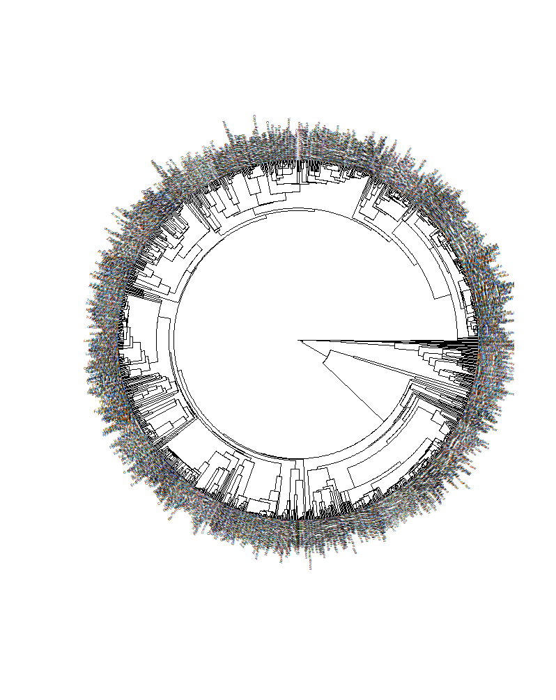
References
Denelle, P., Weigelt, P., & Kreft, H. (2023). GIFT—An R package to access the Global Inventory of Floras and Traits. Methods in Ecology and Evolution, 00, 1–11. https://doi.org/10.1111/2041-210X.14213.
Weigelt, P., König, C. & Kreft, H. (2020) GIFT – A Global Inventory of Floras and Traits for macroecology and biogeography. Journal of Biogeography, https://doi.org/10.1111/jbi.13623.